Review of Data Types

As in most programming languages, data in R can be stored as different data types. Each data type has different attributes, this makes these data types most useful for specific use cases.

It is important to use the correct data type for the associated use case. Therefore, it is important to understand the data types of a given programming language as the foundation to successfully using that language.

In R, we can check the data type of a given input with the class() function.

Booleans

Booleans are binary, they can be true or false. They can have the values of TRUE/T/1 or FALSE/F/0.

class(TRUE)

[1] "logical"

class(T)

[1] "logical"

# Coercing 1 to boolean data type
class(as.logical(1))

[1] "logical"

Boolean Values Must be Capitalized

class(true)

Error in eval(expr, envir, enclos): object 'true' not found

Explicit Programming

In programming, it is usually preferred to be explicit than implicit. If you can write a value, variable name, column title, function name, etc. in a clear way over an abbreviated way, as an explicit programmer it is better to take an extra second and choose the clear way.

In this case, it would generally be better to use TRUE over T as an explicit programmer.

Following the principles of explicit programming, it is important to annotate your code with comments, which can be inserted using the # symbol in R and/or the Ctrl+Shift+C keyboard shortcut in Rstudio/Posit. In your annotated code, comments should be clear enough for another user to understand your code without you explaining it to them.

Keep explicit programming principles in mind throughout this course and your career.

Numerics

Non-complex numbers are referred to by the class numeric in R. They can have the datatype (or subclass) of 1) double, 2) integer.

Doubles

In R, a double is a floating point number. Therefore they can have a decimal point. These numbers can be positive or negative.

Unlike some other programming languages, in R double is always the default data type of a number. Because doubles are the default value of the class numeric, the class() of a double will be shown as numeric. However, using the typeof() function we can see that these numerics are indeed double by default in R.

class(2)

[1] "numeric"

class(2.5)

[1] "numeric"

class(-2.5)

[1] "numeric"

typeof(2)

[1] "double"

typeof(2.5)

[1] "double"

typeof(-2.5)

[1] "double"

Numerics: Trailing Zeros

Unlike many other programming languages, doubles do not automatically display trailing zeros. This can make it a bit more challenging for the user to keep track of what is a double and what is an integer. In reality though, by default in R a number will have two trailing zeros (hence the name “double”) in storage even if these zeros are not displayed,

a <- 2
typeof(a)

[1] "double"

[1] 2

Integers

Integers are whole numbers. They 1) cannot have a decimal point and 2) can be positive or negative.

To specify an integer, include an L following the number.

class(as.integer(2))

[1] "integer"

class(2L)

[1] "integer"

class(-2L)

[1] "integer"

In R, integers are numerics, but numerics are not necessarily integers. That is because numerics can also be doubles.

is.integer(2L)

[1] TRUE

is.numeric(2L)

[1] TRUE

is.integer(2.0)

[1] FALSE

is.numeric(2.0)

[1] TRUE

is.double(2.0)

[1] TRUE

Strings

Strings are how you represent text in R. Note that numbers can indeed be represented in text form.

class("two")

[1] "character"

class("2")

[1] "character"

class(as.character(2))

[1] "character"

Other Data Types

There are other data types in R (single,complex, raw), however we will not cover these at this time.

Data Structures in R

Vectors

Each of the above examples involves a single number or string. We can assign these to an object name.

scalar_1 <- 3
scalar_1

[1] 3

Object Name Assignment Requirements and Convention

Note that in R object names are 1) case-sensitive and 2) cannot include spaces

It is convention in R as well as many other programming languages to begin mutable object names with a lower-case letter

Vectors and Scalars in R

Note that unlike many other programming languages, technically even scalars are actually vectors in R. Under the hood, c(1) and 1 are both identical in R, they are both stored and treated as c(1).

We can combine multiple scalars into a vector data structure. Vectors are

1-dimensional
Contain only one data type

scalar_2 <- 2

vector_1 <- c(scalar_1, scalar_2)
vector_1

[1] 3 2

vector_1 <- c(scalar_1, scalar_2, 3)
vector_1

[1] 3 2 3

Automatic Coercion: Vectors vs. Lists

Note that because vectors can only contain one data type, if more than one data type is present they will all be automatically coerced to the same data type using the following hierarchy.

\[ character\ \leftarrow \ double\ \leftarrow \ integer\ \leftarrow \ logical \]

vector_1 <- c(scalar_1, scalar_2, "1")
vector_1

[1] "3" "2" "1"

vector_1 <- c(scalar_1, scalar_2, TRUE)
vector_1

[1] 3 2 1

In order to avoid this automatic coercion, you can use the data structure list in R

list_a <- list(scalar_1, scalar_2, "1")
list_a

[[1]]
[1] 3

[[2]]
[1] 2

[[3]]
[1] "1"

class(list_a)

[1] "list"

list_b <- list(scalar_1, scalar_2, TRUE)
list_b

[[1]]
[1] 3

[[2]]
[1] 2

[[3]]
[1] TRUE

class(list_b)

[1] "list"

Matrices

The data structure matrices in R are similar to vectors and also can only contain a single data type. However, matrices are 2-dimensional. If you construct a matrix from vectors, you can think of vectors like columns in a matrix.

Matrices can be constructed using the matrix() method.

Caution:

Every row in a matrix must have the same number of columns
Every column in a matrix must have the same number of rows

vector_2 <- c(6, 5, 4)

matrix_1 <- matrix(c(vector_2, vector_1))
matrix_1

     [,1]
[1,]    6
[2,]    5
[3,]    4
[4,]    3
[5,]    2
[6,]    1

matrix_1 <- matrix(c(vector_2, vector_1), ncol = 2)
matrix_1

     [,1] [,2]
[1,]    6    3
[2,]    5    2
[3,]    4    1

class(matrix_1)

[1] "matrix" "array"

Arrays in R

Note that an **array** in R is similar to a matrix but can be comprised of any number of dimensions more than 1, whereas a matrix is comprised of exactly 2 dimensions.

Matrices can also be constructed using the cbind() and/or rbind() methods.

matrix_1 <- cbind(vector_2, vector_1)
matrix_1

     vector_2 vector_1
[1,]        6        3
[2,]        5        2
[3,]        4        1

matrix_2 <- rbind(vector_2, vector_1)
matrix_2

         [,1] [,2] [,3]
vector_2    6    5    4
vector_1    3    2    1

Matrices can be subset

matrix_1[2,1]

vector_2 
       5

Subsetting in R

Note that subsetting in R begins at 1, not 0. This may be different than other programming languages you are used to.

Automatic Coercion: Matrices

Similar to vectors, data types are also coerced in matrices

vector_3 = c("Monday", "Tuesday", "Wednesday")

matrix_2 <- matrix(c(vector_2, vector_1, vector_3), ncol = 3)

matrix_2

     [,1] [,2] [,3]       
[1,] "6"  "3"  "Monday"   
[2,] "5"  "2"  "Tuesday"  
[3,] "4"  "1"  "Wednesday"

class(matrix_2[2,1])

[1] "character"

Data Frames

Data frames in R are similar to matrices in that they are 2-dimensional and row/column lengths must match one another. However there is one major difference, data frames can contain scalars of multiple data types. Because of this attribute to the data frame class, you can use them in the same applications you would use a spreadsheet normally.

In R, you may think of it like: lists are to vectors as data frames are to matrices.

df <- data.frame(column_1 = vector_2, column_2 = vector_1, column_3 = vector_3)
df

  column_1 column_2  column_3
1        6        3    Monday
2        5        2   Tuesday
3        4        1 Wednesday

Just like matrices, data frames can be subset. Note that we avoided coercion with a data frame.

df[2,1]

[1] 5

class(df[2,1])

[1] "numeric"

You can select rows using subsetting

df[df[,1] == 5, ]

  column_1 column_2 column_3
2        5        2  Tuesday

subset(df, column_1 == 5)

  column_1 column_2 column_3
2        5        2  Tuesday

Other Data Structures in R

There are other data structures in R that we will not cover at this time like factors, which are used for categorical variables.

Functions

Functions are actions on an input. They generally produce an output. We have already been using them above, like class(), matrix(), list(), and subset().

Object-Oriented Programming

R is an object-oriented language because everything in R is an object.

By definition in programming, an object is an instance of a class. Classes have certain attributes/properties and specific functions, which are referred to as methods. When an object is created in your code, that object inherits the attributes of the class you assigned it to. These attributes also serve as built-in parameters for the associated methods.

There are also subclasses (child classes) and superclasses (parent classes). If the object you create is a member of subclass, it will inherit all attributes of its class as well as its parent classes.

Object-oriented programming is desirable over procedural programming because it is an efficient, non-redundant way to organize and assign attributes to data. Through object-oriented programming you do not have to assign attributes over and over again each time you initialize an object.

Additionally, by using inheritance the same method can operate differently on an object depending on its specific subclass or superclass which increase readability and reduces complexity. For example:

summary(1:10)

   Min. 1st Qu.  Median    Mean 3rd Qu.    Max. 
   1.00    3.25    5.50    5.50    7.75   10.00

summary(df)

    column_1      column_2     column_3        
 Min.   :4.0   Min.   :1.0   Length:3          
 1st Qu.:4.5   1st Qu.:1.5   Class :character  
 Median :5.0   Median :2.0   Mode  :character  
 Mean   :5.0   Mean   :2.0                     
 3rd Qu.:5.5   3rd Qu.:2.5                     
 Max.   :6.0   Max.   :3.0

Whenever possible in your programming career, it is generally better to write code following object-oriented principles over procedural programming principles.

Writing Your Own Basic Functions

Functions must be defined before they can be called. In R, the definition of a function allows you to:

Name the function
List the required inputs as parameters
Define what the function does

The basic format for writing a function is R is:

Function_Name <- function(parameter1, parameter2) {
  c(parameter1, parameter2)
}

Run the above code chunk, what seems to happen?

When we defined the function, nothing seemed to happen. That is because we must call the function in order to run it.

In order to call the function, we must provide the required parameters as arguments.

Function_Name("argument1", "argument2")

[1] "argument1" "argument2"

Now it is your turn! Write a function called Calculate_Mean() that calculates the mean of vector c(1,2,3,4) using the sum() and length() functions within your function definition.

Note, if you want to check what a function does in R, you can use the help() function or the ?. For example help(length) or ?length().

vector_1 <- c(1,2,3,4)

Calculate_Mean <- function(vector) {
  sum(vector) / length (vector)
}

Calculate_Mean(vector_1)

[1] 2.5

mean(2.5)

[1] 2.5

Functions can also contain default values for parameters following the format:

Function_Name <- function(parameter1, parameter2 = "default") {
  c(parameter1, parameter2)
}

Function_Name("argument1")

[1] "argument1" "default"

These default values can be overwritten by the provided arguments

Function_Name("argument1", "argument2")

[1] "argument1" "argument2"

Write a function that divides each element of vector c(1,2,3,4) by two using a default parameter value of 2.

Divide_by_Two <- function(vector, denominator = 2) {
  vector / denominator
}

Divide_by_Two(vector_1)

[1] 0.5 1.0 1.5 2.0

Now call the same function again without modifying the function itself, but divide each element by 3

Divide_by_Two(vector_1, 3)

[1] 0.3333333 0.6666667 1.0000000 1.3333333

Function Returns

Note what happens by default when we assign the results of function to a new object inside of a function:

vector_1 <- c(1,2,3,4)

Divide_by_Two <- function(vector, denominator = 2) {
  vector_4 <- vector / denominator
}

Divide_by_Two(vector_1)
vector_4

Error in eval(expr, envir, enclos): object 'vector_4' not found

The new object vector_4 is not found outside of the function. This is happening because objects, datasets, and even other functions inside of a function are kept within their own environment.

The base environment is referred to as the “global environment.” The contents of this global environment is displayed in the upper-righthand of Rstudio. We can check that vector_2 is not in the global environment by checking that it is not found in the environment pane. So how do we pass this object from inside the function into the global environment?

R gives you a few options and tries to make this easy for you. Let’s start by clearing the global environment with rm(list=ls()).

rm(list=ls())

Now you can see that the environment pane is empty.

Likely the most straightforward way in R to assign the value produced by a function is to assign the value to an object in the global environment when the function is called:

vector_1 <- c(1,2,3,4)

Divide_by_Two <- function(vector, denominator = 2) {
  vector / denominator
}

vector_4 <- Divide_by_Two(vector_1)
vector_4

[1] 0.5 1.0 1.5 2.0

Super Assignment in R

Another method you may see, but should avoid, is making a global assignment with the “super assignment operator” or “global assignment operator” <<-. Even if an assignment is made inside of a function, this assignment will pass the object globally.

rm(list=ls()) 

vector_1 <- c(1,2,3,4)

Divide_by_Two <- function(vector, denominator = 2) {
  vector_4 <<- vector / denominator
}

Divide_by_Two(vector_1)
vector_4

[1] 0.5 1.0 1.5 2.0

This method is dangerous because if the function is run more than once, the object can unintentionally be reassigned each time

Divide_by_Two <- function(vector, denominator = 2) {
  vector_4 <<- vector / denominator
}

vector_4 <- Divide_by_Two(vector_4)
vector_4

[1] 0.25 0.50 0.75 1.00

vector_4 <- Divide_by_Two(vector_4)
vector_4

[1] 0.125 0.250 0.375 0.500

vector_4 <- Divide_by_Two(vector_4)
vector_4

[1] 0.0625 0.1250 0.1875 0.2500

Explicit Return Statements

As you saw above, unlike some other programming language, R does not require you to explicitly include return statements in order to return values from a function. However, you can still explicitly return values with the return() statement.

This is more in-line with explicit programming principles and can allow you to be certain which values are returned instead of allowing R to automatically make this choice for you.

rm(list=ls()) 

vector_1 <- c(1,2,3,4)

Divide_by_Two <- function(vector, denominator = 2) {
  vector_4 <- vector / denominator
  return(vector_4)
}

vector_4 <- Divide_by_Two(vector_1)
vector_4

[1] 0.5 1.0 1.5 2.0

As a side note, you may also these return statements structured without the return() function in R, as another attempt of R to make returns more automatic

Divide_by_Two <- function(vector, denominator = 2) {
  vector_4 <- vector / denominator
  vector_4
}

Loops

Because R is built around vectors as its most basic unit, R is very well suited for applying functions across rows or columns of a data structure. However, to help with readability the apply family of functions can be used. They are similar to for loops which are also a useful tool.

Write a function to average the values of each numeric column of our matrix_1 <- cbind(c(6,5,4),c(3,2,1)) without using any loop functions.

matrix_1 <- cbind(c(6,5,4),c(3,2,1))

average_columns <- function(M) {
  c(sum(M[,1])/length(M[,1]),sum(M[,2])/length(M[,2]))
  
  # These work as well:  
  # colMeans(M)
  # colSums(M)/nrow(M)
}

average_columns(matrix_1)

[1] 5 2

`for` loops

for loops are used to iterate over the elements of an object. In R the general format of a for loop follows:

for (i in object) {
 print(i)
}

Here is a simple example using our vector_1

for (i in vector_1) {
 print(i)
}

[1] 1
[1] 2
[1] 3
[1] 4

Now write a function that performs the same task as above, but use a for loop. You can use the ncol() and append() functions if you would like.

average_columns <- function(M) {
  placeholder <- c()
  
  for (i in 1:ncol(M)) {
    placeholder <- append(placeholder, sum(M[,i])/length(M[,i]))
  }
  
  placeholder
}

average_columns(matrix_1)

[1] 5 2

apply Family of Functions

`apply()`

Now let’s do the same process with the apply() function instead of our own function, which applies the function to the columns or rows of a multi-dimensional data structure, and the mean() function.

Following the help file, here is the structure: apply(X, MARGIN, FUN, …, simplify = TRUE), where MARGIN = 1 is for rows while MARGIN = 2 is for columns and FUN is any function we want to apply.

apply(matrix_1, MARGIN = 2, mean)

[1] 5 2

Try using apply() to find the square root of each element in our matrix_1

apply(matrix_1, MARGIN = 2, sqrt)

         [,1]     [,2]
[1,] 2.449490 1.732051
[2,] 2.236068 1.414214
[3,] 2.000000 1.000000

Now try using apply() to find the square root of each element in our vector_1

apply(vector_1, MARGIN = 1, sqrt)

Error in apply(vector_1, MARGIN = 1, sqrt): dim(X) must have a positive length

`lapply()`

The lapply() function performs in a similar way, however it can also be used on 1-dimensional data structures, like lists and vectors, whereas apply() would throw an error in those use cases. The output is always a list.

Let’s use it to take the square root of each element of vector_1

lapply(vector_1, sqrt)

[[1]]
[1] 1

[[2]]
[1] 1.414214

[[3]]
[1] 1.732051

[[4]]
[1] 2

`sapply()`

sapply() is similar to lapply() in that it can accept a data structure input of any dimensions. However it does not always return a list, it can return a vector or matrix if it is possible.

Let’s see what happens when we use sapply() on vector_1 instead

sapply(vector_1, sqrt)

[1] 1.000000 1.414214 1.732051 2.000000

Now try the same thing for matrix_1 and compare to the output from apply()

sapply(matrix_1, sqrt)

[1] 2.449490 2.236068 2.000000 1.732051 1.414214 1.000000

Other apply Family Functions

Here is a summary of what we have covered so far.

There are other apply family functions like mapply() and tapply(), however we will not cover those at this time.

It’s worth mentioning that there are other alternatives to the apply family of functions including map() from the purrr(Wickham and Henry 2023) package as well as rowwise(), colwise(), and across() from the dplyr(Wickham et al. 2022) package.

Packages in R

Libraries in R are called packages. These packages contain a suite of specific functions and classes. For example, we will be using the dplyr(Wickham et al. 2022) package in R in this course to wrangle data frames and the ggplot2(Wickham 2016) package for visualizing plots.

To install packages, use the following commands:

install.packages("dplyr")
install.packages("ggplot2")

# Note that "packages" is plural and that the package name is in quotes

Now these packages are installed across R workspaces on your device. However, when you begin your session, you must load your packages into your current workspace.

library("dplyr")

Warning: package 'dplyr' was built under R version 4.3.2


Attaching package: 'dplyr'

The following objects are masked from 'package:stats':

    filter, lag

The following objects are masked from 'package:base':

    intersect, setdiff, setequal, union

library("ggplot2")

Warning: package 'ggplot2' was built under R version 4.3.2

Note that you may see require() used in place of library(). Both of these commands will load the package into your workspace. However, library() produces an error while require() provides just a warning. An error will stop the R script while a warning will not.

The most intuitive way to wrangle data in R is by using the dplyr (Wickham et al. 2023) package which is included in the tidyverse (Wickham et al. 2019) set of packages.

Data-wrangling and the Grammar of Data Manipulation

The grammar of data manipulation is a set of principles and concepts that provide a consistent approach to thinking about data manipulation. It is based on the idea that there are a only small number of fundamental operations in data manipulation, primarily of which are:

Filtering: Filtering a subset of rows based on a criteria.
Selecting: Selecting which columns to include in the output.
Mutating: Ceating new columns or modifying existing ones, usually by manipulating the data in existing columns.
Summarizing: Aggregating data by groups. For example, calculating the mean of a measurement for a certain group.

The dplyr package uses this grammar of data manipulation for data-wrangling in R:

As a tidyverse package, this wrangling can be accomplished in a streamlined fashion using tidyverse pipes %>%. These were originally introduced in the maggritr (Bache and Wickham 2022) tidyverse package but has now been incorporated into other packages as well, like dplyr. To learn how to use pipes, let’s first wrangle data without pipes.

# Construct a simple dataframe

df <- data.frame(column1 = c(1, -2, 3, 7, 33, 1, 4),
                 column2 = c(4, 5, 6, 22, 44, 1, 4),
                 column3 = c(7, 8, 9, 22, 50, 1, 3))

df

  column1 column2 column3
1       1       4       7
2      -2       5       8
3       3       6       9
4       7      22      22
5      33      44      50
6       1       1       1
7       4       4       3

Here we wrangle the data using dplyr without pipes

# Filter for only rows in `column1` containing positive numbers
df_base <- filter(df, column1 > 0)

# Select only the second and third column
df_base <- select(df_base, column2, column3)

# Create another column that has elements that are the sum of columns 2 and 3
df_base <- mutate(df_base, column4 = df_base$column2 + df_base$column3)

df_base

  column2 column3 column4
1       4       7      11
2       6       9      15
3      22      22      44
4      44      50      94
5       1       1       2
6       4       3       7

Here is the basic format of tidyverse pipes in R:

df_out <- df_in %>%
  function(<column_name>) %>%
  function(<row_name>)

Note that the assignment only happens once. Also note that the input object, in this case df_in generally needs to only be provided once. It is implied to be inserted as the first term of the function by the pipe. Therefore following a pipe, these are equivalent: function(df, df$<column_name>) $<=>$ function(df, <column_name>) $<=>$ function(., <column_name>) $<=>$ function(<column_name>)

function(<column_name>)

Compare this to the example above.

Now, rewrite the data-wrangling process above using pipes to create object df_tidyverse

df_tidyverse <- df %>%
  filter(column1 > 0) %>%
  select(column2, column3) %>%
  mutate(column4 = column2 + column3)

df_tidyverse

  column2 column3 column4
1       4       7      11
2       6       9      15
3      22      22      44
4      44      50      94
5       1       1       2
6       4       3       7

Grammar of Graphics in R

Just like we covered the Grammar of Data Manipulation last week when we introduced the dplyr package (Wickham et al. 2022), plots can also be de-composed into grammatical elements (Wilkinson 2012) to help intuitively build plots from three primary components:

Data
Geoms: Geometric options
Coordinate system (default Cartesian)

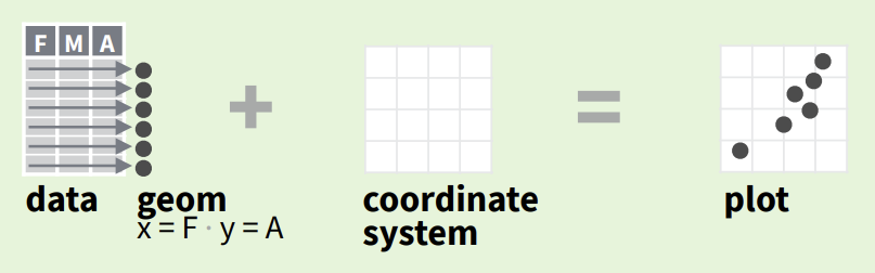
Variables in the dataset can be mapped to one another using mapping aesthetics (aes()) . For example, default mapping aes(x = variable_1, y = y_variable_2) maps the first variable to x-axis and second variable to the y-axis.

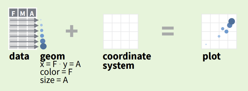
Other common mappings include:

color: assigns a color to each category
size: scales the size of points or lines based on numeric variable
shape: assigns a shape to each category
fill: fills the interior of points or shapes based on categorical variable

Similar to the `%>% pipe operator in dplyr, ggplot components are added to one another sequentially with +

# Create a ggplot object from the data 
ggplot(data = df, aes(<mapping> = <variable_1>, <mapping> = <variable_2>)) +
  # Create a geometric object
  geom_<type>() +
  # Add labels
  labs(title = "Title", x = "X-axis", y = "Y-axis")

Now try with our dataset df_tidyverse. Create a scatter plot of column2 vs column3 with the size of the points scaled by column4. Add a title and label the axes.

ggplot(data = df_tidyverse, aes(x = column2, y = column3, size = column4)) +
  geom_point() +
  labs(title = "Scatter Plot of column2 vs column3",
       x = "Column 2",
       y = "Column 3",
       size = "Sum of Column 2 and 3")

With these intuitive lines of code, we are able to generate a useful plot. What do you think the plot might be indicating?

Now change column4 to be represented by color instead of size. This is easily altered using ggplot2.

ggplot(data = df_tidyverse, aes(x = column2, y = column3, color = column4)) +
  geom_point() +
  labs(title = "Scatter Plot of column2 vs column3",
       x = "Column 2",
       y = "Column 3",
       size = "Sum of Column 2 and 3")

This guide will help you to further customize your plots using ggplot2 including the other common components labels, scale, themes, and stats

References

Bache, Stefan Milton, and Hadley Wickham. 2022. “Magrittr: A Forward-Pipe Operator for r.” https://CRAN.R-project.org/package=magrittr.

Stevens, Martin Henry Hoffman. 2009. A Primer of Ecology with r. Springer.

Wickham, Hadley. 2016. “Ggplot2: Elegant Graphics for Data Analysis.” https://ggplot2.tidyverse.org.

Wickham, Hadley, Mara Averick, Jennifer Bryan, Winston Chang, Lucy D’Agostino McGowan, Romain François, Garrett Grolemund, et al. 2019. “Welcome to the Tidyverse” 4: 1686. https://doi.org/10.21105/joss.01686.

Wickham, Hadley, Romain François, Lionel Henry, and Kirill Müller. 2022. Dplyr: A Grammar of Data Manipulation.

Wickham, Hadley, Romain François, Lionel Henry, Kirill Müller, and Davis Vaughan. 2023. “Dplyr: A Grammar of Data Manipulation.” https://CRAN.R-project.org/package=dplyr.

Wickham, Hadley, and Lionel Henry. 2023. Purrr: Functional Programming Tools. https://CRAN.R-project.org/package=purrr.

Wilkinson, Leland. 2012. The Grammar of Graphics. Springer.

Review of Data Types

Booleans

Numerics

Doubles

Integers

Strings

Other Data Types

Data Structures in R

Vectors

Matrices

Data Frames

Other Data Structures in R

Functions

Writing Your Own Basic Functions

Function Returns

Loops

for loops

apply Family of Functions

apply()

lapply()

sapply()

Other apply Family Functions

References

`for` loops

`apply()`

`lapply()`

`sapply()`